Assumptions in Linear regression

Assumptions in linear regression refer to a set of conditions or requirements that need to be satisfied for the regression model to be valid and for the statistical inference to be reliable. These assumptions help ensure that the estimates and inferences derived from the model are meaningful and accurate.

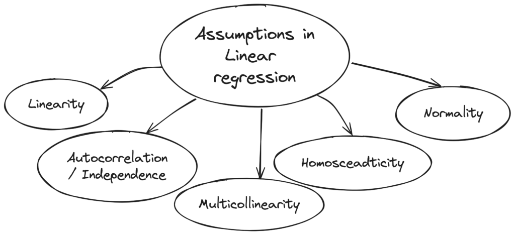
Linearity

The assumption of linearity in linear regression refers to the relationship between the independent variable(s) and the dependent variable being linear. This means that the effect of a change in the independent variable(s) on the dependent variable is constant across all levels of the independent variable(s).

Autocorrelation / Independence

The assumption of no autocorrelation (also known as independence of errors) in linear regression refers to the condition that the residuals or errors of the model are not correlated with each other.

Autocorrelation occurs when the residual of an observation is correlated with the residual of another observation, leading to a pattern in the residuals. This pattern may indicate that there is some important variable that is not included in the model, or that the model is misspecified in some way. This is also observed in time-series data.

Autocorrelation can be detected using a plot of the residuals against the order of the observations, known as a correlogram. If there is significant autocorrelation in the residuals, it can be corrected using techniques such as adding additional variables to the model or using a different modeling approach such as time series analysis.

Multicollinearity

Multicollinearity occurs when two or more predictor variables in a multiple regression model are highly correlated with each other, making it difficult to determine the separate effects of each variable on the dependent variable.

One of the primary issues with multicollinearity is that the coefficients for the correlated variables become unstable, meaning that small changes in the data can result in large changes in the estimated coefficients. This makes it difficult to interpret the results of the regression analysis and can lead to incorrect conclusions about the relationships between the predictor variables and the dependent variable.

To detect multicollinearity you can follow any of the following techniques-

1. Calculate the correlation matrix among the predictor variables. Correlations above a certain threshold (e.g., 0.7 or 0.8) may indicate multicollinearity
2. Tolerance
   Tolerance = 1 / VIF
   VIF = 1 / (1 – R²)
   
   where R² is the coefficient of determination obtained from regressing the predictor variable of interest on all the other predictor variables in the model.
   The VIF measures the extent to which the variance of the estimated regression coefficient is inflated due to multicollinearity. A VIF of 1 indicates no multicollinearity, while a VIF of greater than 1 suggests that there is some degree of multicollinearity.
   
   Tolerance values range from 0 to 1, with a tolerance of 1 indicating no multicollinearity and a tolerance of 0 indicating perfect multicollinearity (i.e., one predictor variable is a linear combination of one or more other predictor variables). In general, a tolerance value less than 0.1 (or a VIF greater than 10) is considered to be indicative of problematic multicollinearity.
3. You can also use diagnostic plots, such as scatterplots of the predictor variables against each other, to visualize the presence of multicollinearity.
   
   To address multicollinearity, you can consider several options. One option is to remove one or more of the correlated predictor variables from the model. Another option is to combine the correlated variables into a single variable through techniques such as principal component analysis. Finally, you can use regularization techniques such as ridge regression or lasso regression, which can help to reduce the impact of multicollinearity on the regression coefficients.

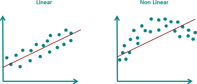
Homosceadticity

Homoscedasticity, also known as homogeneity of variance, is an assumption of linear regression that states that the variance of the errors (or residuals) is constant across all levels of the predictor variable(s). In other words, the spread of the residuals is the same throughout the range of the predictor variable(s).

When the assumption of homoscedasticity is violated, the spread of the residuals may be larger or smaller for certain values of the predictor variable(s), leading to biased or inefficient estimates of the regression coefficients, and unreliable predictions.

There are several graphical methods to assess homoscedasticity, such as residual plots or scatterplots of the residuals against the predicted values. In a scatterplot of the residuals against the predicted values, a pattern of increasing or decreasing spread of the residuals as the predicted values increase suggests heteroscedasticity, while a constant spread of the residuals across the range of the predicted values suggests homoscedasticity.

If heteroscedasticity is detected, there are several options to address the issue. One option is to transform the response variable or predictor variable(s) using a mathematical function, such as logarithmic or square root transformation, to reduce the impact of outliers or extreme values. Another option is to use weighted least squares regression, which assigns different weights to the observations based on their variance, to obtain more accurate and efficient estimates of the regression coefficients. Alternatively, one can use robust regression methods, such as the Huber or Tukey bisquare estimators, which are less sensitive to outliers and deviations from normality and can provide more robust estimates of the regression coefficients.

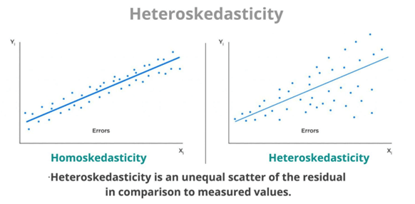
Normality

Normality states that the residuals (or errors) of the regression model should be normally distributed. In other words, the distribution of the residuals should be symmetric and bell-shaped around zero.

The normality assumption is important because it allows us to use statistical inference techniques, such as hypothesis testing and confidence intervals, that rely on the assumption of normality. When the normality assumption is not met, the estimates of the regression coefficients and their standard errors may be biased, and the results of hypothesis testing may be inaccurate or misleading.

To assess the normality assumption, we can use several graphical methods, such as a histogram or a normal probability plot of the residuals. A histogram of the residuals should show a symmetric and bell-shaped distribution around zero. A normal probability plot of the residuals should show a roughly linear pattern, indicating that the residuals follow a normal distribution.

If the normality assumption is violated, there are several options to address the issue. One option is to transform the response variable or predictor variable(s) using a mathematical function, such as logarithmic or square root transformation, to make the residuals more normally distributed. Another option is to use non-parametric regression methods, such as quantile regression or robust regression, which are less sensitive to deviations from normality and can provide more accurate and robust estimates of the regression coefficients. Additionally, one can consider using techniques such as bootstrapping or permutation tests, which do not rely on the assumption of normality to perform inference.