Linear Regression

Let’s start with our first algorithm of machine learning – Linear Regression. This algorithm is used to predict a target that is continuous like the price of the house, the temperature of a place, the rating of a movie, etc. But before proceeding with the algorithm, let’s understand the rough working of any supervised machine learning algorithm.

An algorithm mainly consists of a hypothesis i.e. the function the model will apply to the features to get the output. We have a cost function that determines the accuracy of the model at any given time during the training. It’s reasonable to say that the ultimate target of learning is to minimize the cost. But how does the model minimize the cost? Using the Optimiser. An optimizer is an algorithm that is used to update the parameters of a machine learning model during training to minimize the loss function. The optimizer determines the direction and magnitude of the updates to the model’s parameters in each iteration of the training process. This was a rough idea of how any supervised machine-learning algorithm works. Now let’s try to understand one algorithm in detail.

Types of Linear Regression

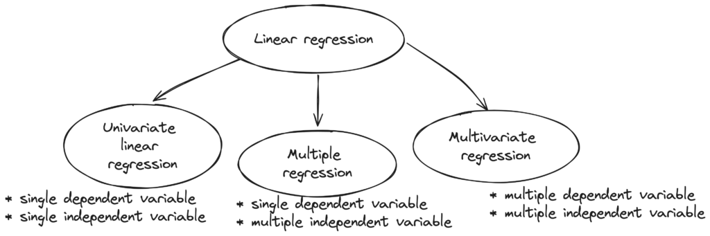
Univariate linear regression

Univariate linear regression means that there is a single feature and a single target. Let’s say you’ve to predict house price based on the size of the plot the house is constructed on. Let’s look at the hypothesis function for it.

Hypothesis function

$\hat{y} = h_{\theta}(x) = \theta_{0} + \theta_{1}x$

Here x is the size of the plot and y cap is the price. θ’s are the model parameters.

vectorized form:

$\hat{y} = h_{\theta}(x) = \theta^{T}x$

Cost function

$J(\theta_{0}, \theta_{1}) = \frac{1}{2m} \sum_{i=1}^{m}(\hat{y}_{i} - y_{i})^{2}$

this is the function that calculates the error of the prediction while training. y cap is the predicted price and y is the actual price.

squared error function or mean squared error
1/2 is there to cancel the constant in derivative while computing gradient descent

Gradient descent optimizer

Repeat until convergence:

$\theta_{j} := \theta_{j} - \alpha \frac{\partial }{\partial \theta_{j}} J(\theta_{0}, \theta_{1})$

α (learning rate): The learning rate is a hyperparameter that determines how much the weights of a model are updated during training. It is a scaling factor that controls how quickly the model learns from the data. If the learning rate is too small, the model may take a long time to converge, or it may get stuck in a suboptimal solution. On the other hand, if the learning rate is too high, the model may overshoot the optimal solution and oscillate around it or diverge. It is typically set through trial and error.

The derivative of the cost function determines the direction and magnitude of the update of θ. Let’s try to understand what exactly the optimizer does to model parameters.

This is a graph of the loss function with respect to θ.

Initially, we got a random value of θ, which means that we could be anywhere on this graph, but the final target is to reach to minimize the loss which is to reach the bottom of this graph (red pointer). The optimizer updates the θ’s iteratively such that the final value is at the bottom.