Loss functions

A loss function is a mathematical function that measures the difference between the predicted output of a model and the actual output. The goal of training a machine learning model is to minimize the value of the loss function so that the predicted output of the model is as close as possible to the actual output.

There are many types of loss functions, each with its own strengths and weaknesses depending on the problem at hand. Choosing an appropriate loss function is an essential step in training a machine learning model. Let us start with some loss functions used in regression

Feasibility condition for a loss function.

Feasibility conditions are a set of conditions that a loss function must meet in order to be considered a valid and useful loss function. These conditions vary depending on the problem at hand and the characteristics of the data. Some common feasibility conditions for a loss function include:

Convexity: A loss function should be convex, meaning that it should have a single global minimum that can be found by an optimization algorithm. This guarantees that the optimization problem has a unique solution and is stable.
Differentiability: A loss function should be differentiable, meaning that the gradient of the loss function with respect to the model parameters can be calculated. This allows the optimization algorithm to update the model parameters in the direction of the gradient.
Continuity: A loss function should be continuous, meaning that small changes in the input should result in small changes in the output. This allows the optimization algorithm to converge to a solution.
Boundedness: A loss function should be bounded, meaning that there should be a finite upper limit to the loss function’s value. This ensures that the optimization algorithm does not diverge to infinity.
Scale-invariant: A loss function should be scale-invariant, meaning that it should give the same result regardless of the scale of the input data. This allows the optimization algorithm to converge to the same solution regardless of the scale of the data.
Problem-specific: The loss function should be appropriate for the specific problem at hand, for example, for a regression problem, mean squared error is a good choice, while for a classification problem, cross-entropy loss function is a good choice.

Loss function in regression

Mean squared error

$MSE = \frac{1}{n}\sum_{i=1}^{n}(y_{i} - \hat{y_{i}})^{2}$

Where y_i is the actual output and ŷ_i is the predicted output.
When the target distribution is gaussian.
Squaring makes errors more significant for large-magnitude errors.
Mostly the output layer has a single node and linear activation function.

Mean squared logarithmic error

$MSLE = \frac{1}{n}\sum_{i=1}^{n}(log(y_{i} + 1) - log(\hat{y_{i}} + 1))^{2}$

When the target has a spread of values and while predicting a large value, we don’t want to punish the error with a square.
Since log has a negative value in the range (0, 1), we add 1 so that the range is (0, ∞)

Mean absolute error

$MSE = \frac{1}{n} \sum_{i=1}^{n} |y_{i} - \hat{y_{i}}|$

The distribution of the target is mostly gaussian with some outliers.

Loss function for Binary classification

Binary cross entropy loss

$BCE = -\frac{1}{n}\sum_{i=1}^{n}y_{i}log(\hat{y_{i}}) + (1 - y_{i})log(1 - \hat{y_{i}})$

This loss function is used when the output of a model is a probability between 0 and 1. Let’s break down and understand the cost function.

$Cost(y) =\begin{cases}-log(\hat{y_{i}})& \text{ if } y= 1\\-log(1 - \hat{y_{i}})& \text{ if } y= 0\end{cases}$

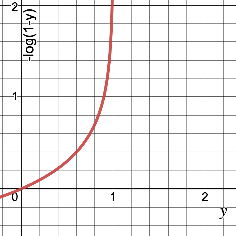
After plotting the cost function for both the values of y, observe that the cost is higher when predicted y is closer to 0 and actual y is closer to 1 and similarly when actual y = 0, the cost is high when prediction is close to 1.

Hinge loss

$hinge = \frac{1}{n} \sum_{i=1}^{n} max(0, 1-y.\hat{y})$

The hinge loss is commonly used in SVMs because it is a convex function, which makes it easy to optimize using gradient descent. It is also robust to outliers and is less sensitive to the choice of parameters than other loss functions, such as the mean squared error.

Hinge loss is also used in other machine learning models such as in deep learning to train models with large margin.

Let’s look at the graph and understand the function

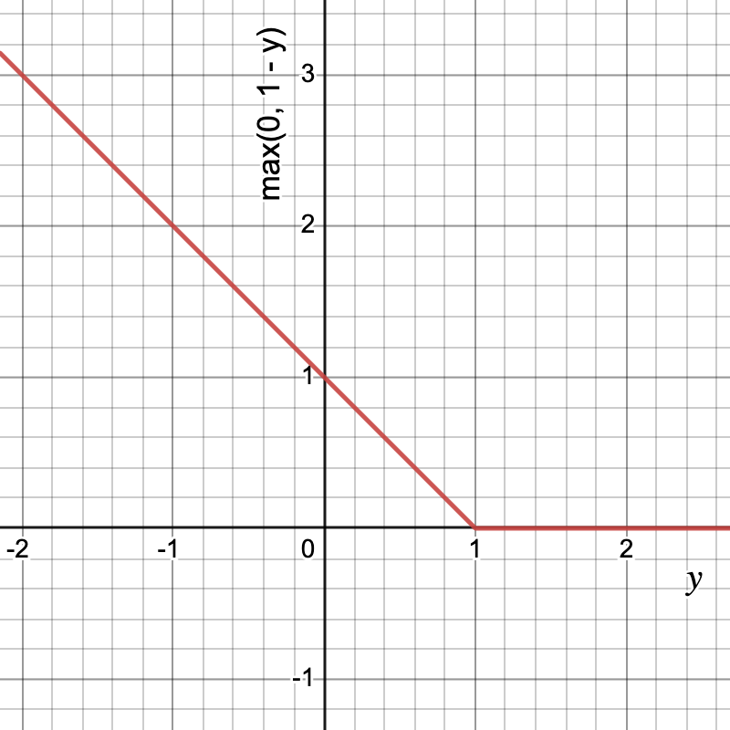
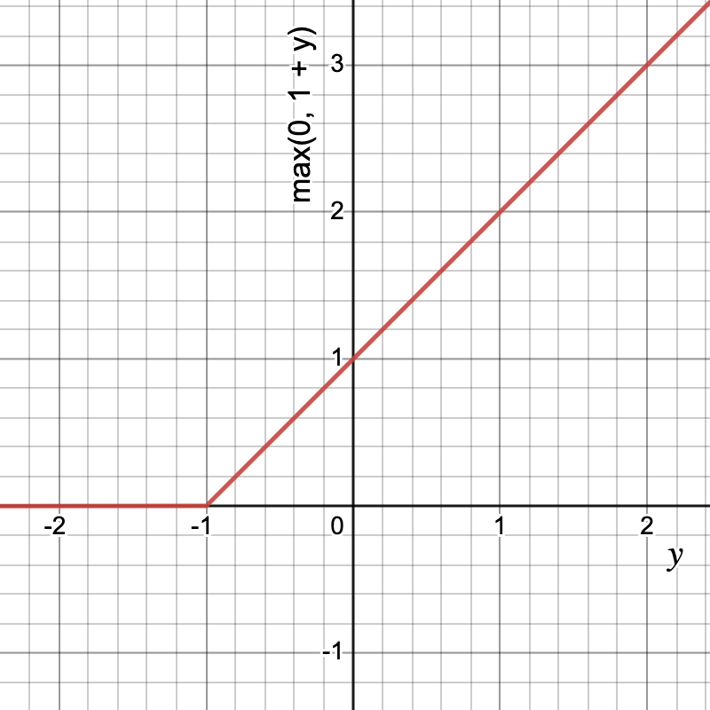
This function is used when y ∈ {-1, 1}.