Decision Tree - ID3 - akashnotes

Introduction

ID3 stands for Iterative Dichotomiser 3 and is named such because the algorithm iteratively (repeatedly) dichotomizes(divides) features into two or more groups at each step.

ID3 uses a top-down greedy approach to build a decision tree. In simple words, the top-down approach means that we start building the tree from the top and the greedy approach means that at each iteration we select the best feature at the present moment to create a node.

Most generally ID3 is only used for classification problems with nominal features.

Dataset

Let’s take a COVID-19 sample data to understand this algorithm better. The target column is Infected – YES/NO and the columns to make decisions are Fever, Cough, and Breathing issues.

ID	Fever	Cough	Breathing Issue	Infected
1	No	No	No	No
2	Yes	Yes	Yes	Yes
3	Yes	Yes	No	No
4	Yes	No	Yes	Yes
5	Yes	Yes	Yes	Yes
6	No	Yes	No	No
7	Yes	No	Yes	Yes
8	Yes	No	Yes	Yes
9	No	Yes	Yes	Yes
10	Yes	Yes	No	Yes
11	No	Yes	No	No
12	No	Yes	Yes	Yes
13	No	Yes	Yes	No
14	Yes	Yes	No	No

Metrics

ID3 uses Information Gain or Gain to find the best feature.

Information Gain calculates the reduction in the entropy and measures how well a given feature separates or classifies the target classes. The feature with the highest Information Gain is selected as the best one.

In the case of binary classification (where the target column has only two types of classes), entropy is 0 if all values in the target column are homogenous(similar) and will be 1 if the target column has equal number values for both classes.

$Entropy(S) = -\sum_{i=1}^{n} p_{i} * log_{2}(p_{i})$

where
S : dataset
n: total number of classes
p_i: the probability of class i or ratio of “number of rows with class i in the target column” to the “total number of rows” in the dataset.

Information gain for a column A is calculated as:

$IG(S, A) = Entropy(S) - \sum\frac{|S_{v}|}{|S|} * Entropy(S_{v})$

where Sᵥ is the set of rows in S for which the feature column A has value v, |Sᵥ| is the number of rows in Sᵥ, and |S| is the number of rows in S.

Algorithm

Calculate the Information Gain of each feature.
Since all rows don’t belong to the same class, split the dataset S into subsets using the feature for which the Information Gain is maximum.
Make a decision tree node using the feature with the maximum Information gain.
If all rows belong to the same class, make the current node as a leaf node with the class as its label.
Repeat for the remaining features until we run out of all features, or the decision tree has all leaf nodes.

Implementation

Now let us look at our dataset and see how we can construct a decision tree using out covid dataset.

1. Calculate the Information Gain of each feature.

IG calculation for Fever:
In this feature, 8 rows have the value YES, and 6 rows have the value NO.

ID	Fever	Cough	Breathing Issue	Infected
2	Yes	Yes	Yes	Yes
3	Yes	Yes	No	No
4	Yes	No	Yes	Yes
5	Yes	Yes	Yes	Yes
7	Yes	No	Yes	Yes
8	Yes	No	Yes	Yes
10	Yes	Yes	No	Yes
14	Yes	Yes	No	No

As shown above, in the 8 rows with YES for Fever, there are 6 rows having target value YES and 2 rows having target value NO.

ID	Fever	Cough	Breathing Issue	Infected
1	No	No	No	No
6	No	Yes	No	No
9	No	Yes	Yes	Yes
11	No	Yes	No	No
12	No	Yes	Yes	Yes
13	No	Yes	Yes	No

As shown above, in the 6 rows with NO, there are 2 rows having target value YES and 4 rows having target value NO.

Entropy of dataset:

$Entropy(S) = - \frac{8}{14} * log_{2}(\frac{8}{14}) - \frac{6}{14} * log_{2}(\frac{6}{14})$

Information gain for fever:

total rows
|S| = 14

For v = YES, |Sᵥ| = 8
Entropy(Sᵥ) = - (6/8) * log₂(6/8) - (2/8) * log₂(2/8) = 0.81

For v = NO, |Sᵥ| = 6
Entropy(Sᵥ) = - (2/6) * log₂(2/6) - (4/6) * log₂(4/6) = 0.91

# Expanding the summation in the IG formula:
IG(S, Fever) = Entropy(S) - (|Sʏᴇꜱ| / |S|) * Entropy(Sʏᴇꜱ) - 
(|Sɴᴏ| / |S|) * Entropy(Sɴᴏ)

∴ IG(S, Fever) = 0.99 - (8/14) * 0.81 - (6/14) * 0.91 = 0.13

Similarly, we can calculate IG for

IG(S, Cough) = 0.04
IG(S, BreathingIssues) = 0.40

Here we can see that the Breathing issue feature has higher information gain thus we can split our dataset using this feature at the root node.
After the split this is what our tree will look like:

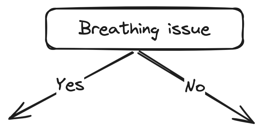
Now we take the left node (with the Breathing issue as YES) and calculate the same for the remaining features (Cough and Fever). Note that the data in the left node will only be for the rows with the Breathing issue as YES.

IG(Sʙʏ, Fever) = 0.20
IG(Sʙʏ, Cough) = 0.09

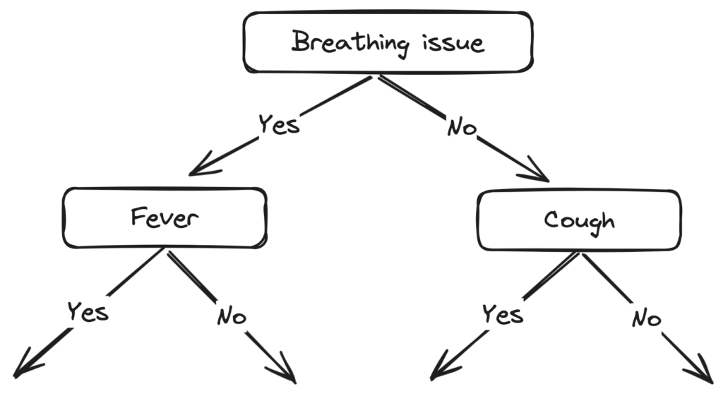
IG of Fever is greater than that of Cough, so we select Fever as the left branch of Breathing Issues:

Our tree now looks like this:

Next, we find the feature with the maximum IG for the right branch of Breathing Issues. But, since there is only one unused feature left we have no other choice but to make it the right branch of the root node.

So our tree now looks like this:

For the leaf nodes, we just take the mode of the data at every leaf node and assign the labels.

For the left leaf node of Fever, we see the subset of rows from the original data set that has Breathing Issues and Fever both values as YES.

ID	Fever	Cough	Breathing Issue	Infected
2	Yes	Yes	Yes	Yes
4	Yes	No	Yes	Yes
5	Yes	Yes	Yes	Yes
7	Yes	No	Yes	Yes
8	Yes	No	Yes	Yes

Since all the values in the target column are YES, we label the left leaf node as YES, but to make it more logical we label it Infected.

After doing the same for all the leaves this is what the final tree looks like –

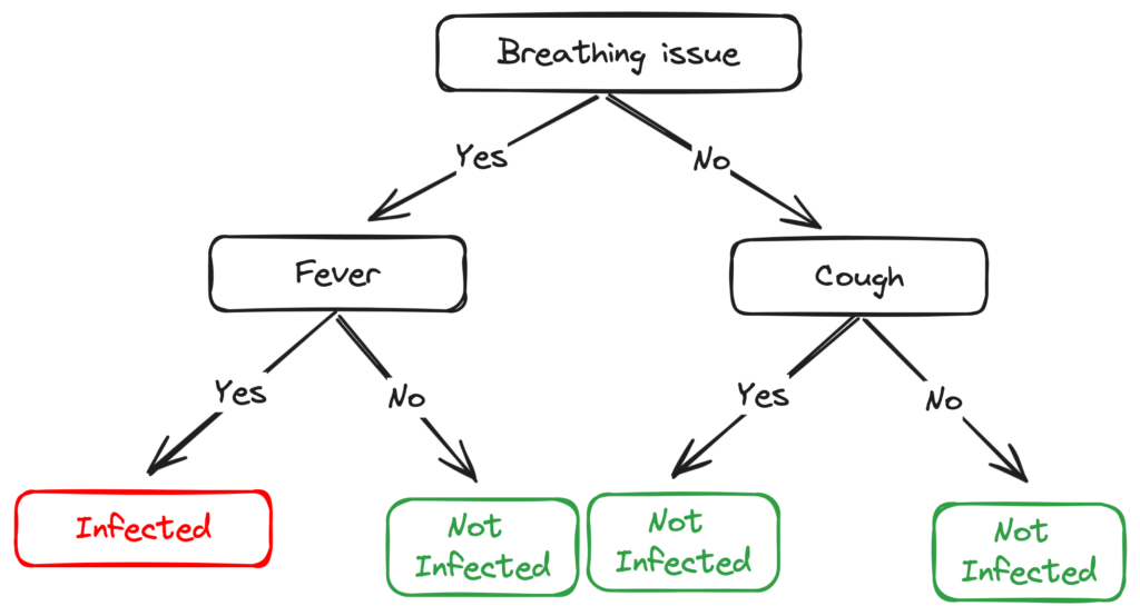
The right node of Breathing issues is as good as just a leaf node with the class ‘Not infected’. This is one of the Drawbacks of ID3, it doesn’t do pruning.

Pruning is a mechanism that reduces the size and complexity of a Decision tree by removing unnecessary nodes.

Code

Data link: Link

Decision Tree – ID3