Convolution neural networks or CNN is a revolutionary algorithm used in modeling image data. Images are nothing but numbers, very similar to any other tabular data, but with a few fundamental differences. One, Image pixels are associated with nearby pixels. If I provide you with a long list of image pixel values, it might mean nothing, but when you know the nearby pixels of an area, it forms some meaningful property of the image, so it’s very important to understand the relation of pixels nearby each other. Second, there are a lot of pixels in an image, so if we link one input node (pixel) with one edge to the next layer, we might end up having a very large number of trainable parameters. So CNN used something called parameter sharing to optimize that.
Convolution layer
Convolution neural networks are designed to extract features from images to differentiate one image from another. The preprocessing required in this type of network is very less compared to other algorithms that work on images.
The major advantage of CNN or convolution layer is Spatial dependency. Spatial Dependency means a pixel’s value is influenced by a nearby pixel’s value in the image. This is because generally, they all belong to the same color because they are from the same object. There are more advantages of CNN but let’s dive into the algorithm first.
Algorithm
You might know that image is nothing but a collection of pixels i.e. a collection of numbers. Typically an image has 3 layers (Red, Green, and Blue) but here to introduce convolution we’ve taken a single-layered image or a GrayScale image.
Let’s say we have a small image as follows.
[[0.1, 0.2, 0.3],
[0.4, 0.5, 0.6],
[0.7, 0.8, 0.9]]
and a kernel as:
[[1, 0, 1],
[0, 1, 0],
[1, 0, 1]]
Now for one convolution operation, we take the sum of products pixel-wise i.e.
0.1×1 + 0.2×0 + 0.3×1 + 0.4×0 + 0.5×1 + 0.6×0 + 0.7×1 + 0.8×0 + 0.9×1 = 2.5
and this is the output of one operation. In the convolution layer, we make multiple such operations over the image to get the output. Something like this:
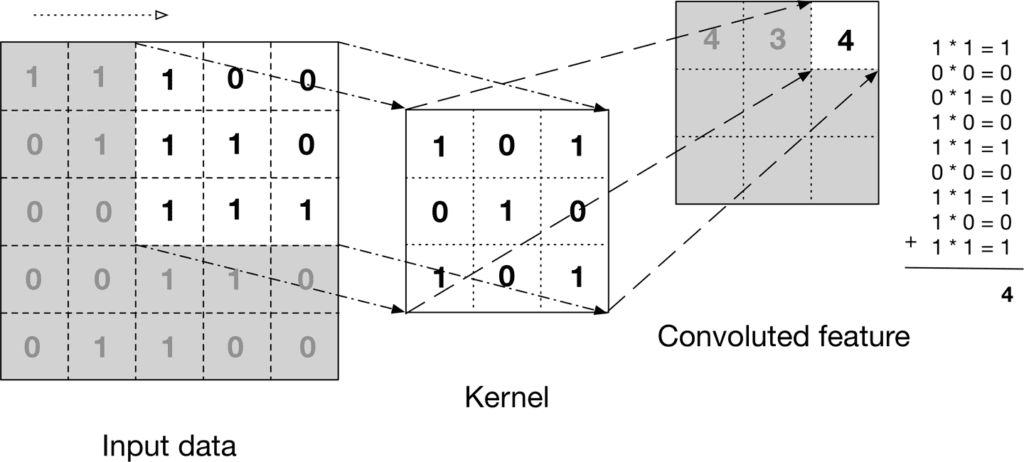
Here is another example of how the convolution layer is performed on an image to get a feature map.
Let’s observe the dimension of the image and feature map (output after applying the convolution layer). For an image of 5×5 and a filter of 3×3, we got a feature map of 3×3. Can we devise a formula for output image size given the input image dimension and kernel size?

so for our example i.e. input_dimension = 5 and kernel_dimension = 3 we have output size 5-3+1 = 3.
Padding
Now you can see the border and the corner of the image had lesser operation than other parts of the image. Also, the dimension is constantly reducing, which limits the number of times we can apply convolution operation. To avoid this we use padding, a very simple concept – add 0 values to the border of the image.
Image before padding
[[0.1, 0.2, 0.3],
[0.4, 0.5, 0.6],
[0.7, 0.8, 0.9]]
Image after padding of one pixel with 0s.
[[0, 0,  0,   0,   0],
[0, 0.1, 0.2, 0.3, 0],
[0, 0.4, 0.5, 0.6, 0],
[0, 0.7, 0.8, 0.9, 0],
[0, 0,   0,   0,   0]]
Strides
We saw in the above convolution operation that the kernel moves one pixel to the right and bottom while the convolution operation. What if we increase the pixel gap between two convolution operations? The following image will it more clear.
This is a convolution operation on a padded image (dotted lines are padding) with strides as 2. Now can you guess why we need to increase the stride? Yes, you are right – to decrease the image size. This is generally followed when the input image size is quite large and strides = 1 adds similar information to the output feature map.
Now you see we need a new formula to calculate output image size:
